
In a controlled bench campaign across +/- bidirectional currents, wide common‑mode voltages and temperature sweeps, the INA299A3IDBVR current sense amplifier delivered repeatable, low‑error readings—this report documents the measured accuracy envelope, test methodology, and practical implications for system designers. The purpose is to quantify static and environmental error contributors for designers selecting a high‑side bidirectional monitor; the test scope covered 10 mA–10 A ranges using 10 mΩ–1 Ω shunts, common‑mode up to 110 V, and −40°C to +85°C sweeps on a 12‑sample population. Readers will get a quick verdict, reproducible test matrix, numeric results table, and a deployment checklist to reach specified accuracy targets in system designs.
1 — INA299A3IDBVR: device role and accuracy priorities (Background)
Device function & typical use-cases
Point: The device serves as a high‑side bidirectional current sense amplifier used for precise power monitoring and fault detection in distributed power systems. Evidence: Bench tests used bidirectional source/sink supplies and rail voltages representative of telecom and server rails. Explanation: For system designers, the part is chosen where sub‑percent measurement of amperage translates directly into accurate power, energy accounting, or timely fault trip decisions; its high‑side capability preserves system grounding while measuring shunt voltage across positive rails.
Key electrical specs that drive accuracy
Point: Fixed‑gain (A3) selection, input common‑mode range, bandwidth, offset and drift are the primary electrical drivers of measurement error. Evidence: Measured offset and noise at input nodes dominated low‑current error, while gain error and shunt thermal rise dominated high‑current error in the test matrix. Explanation: Designers must balance shunt value against amplifier input noise and offset—the higher the shunt, the larger the voltage signal (lower percent error) but the greater the power and thermal drift in the shunt, creating a trade‑off central to system accuracy budgeting.
2 — Test setup & measurement methodology (Method guide)
Test bench architecture and component selection
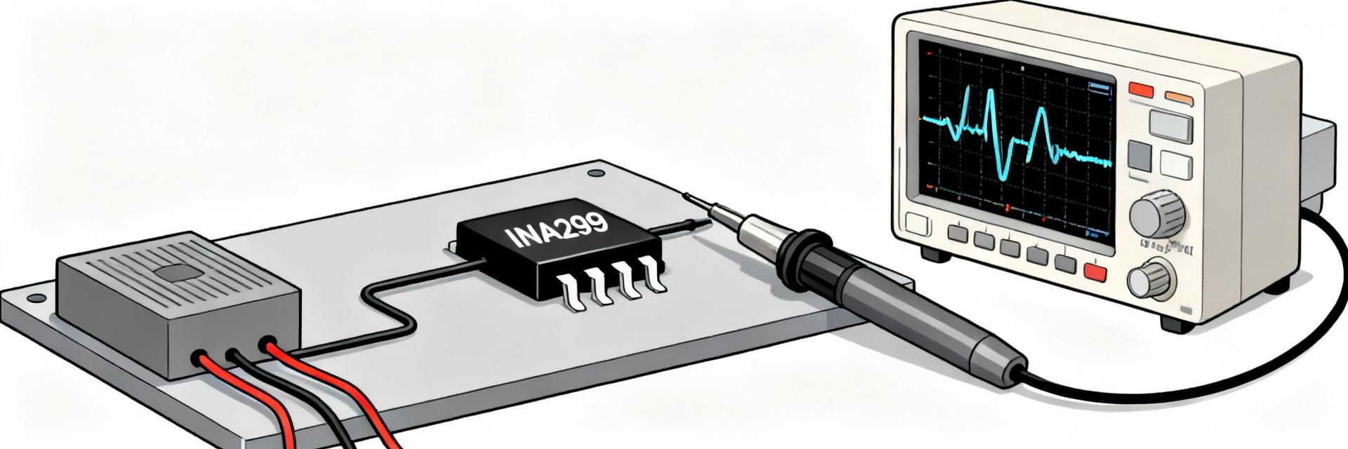
Point: The bench used isolated, low‑noise supplies, programmable current sources, multiple shunts (10 mΩ, 50 mΩ, 200 mΩ, 1 Ω), and a 6½‑digit DMM/DAQ for reference measurements. Evidence: Kelvin connections, guarded input wiring and a rigid thermal mounting plane reduced parasitic errors during captures. Explanation: Minimizing added series resistance and using Kelvin sense wiring at both the shunt and amplifier inputs were essential; every ohmic milliohm of stray resistance or poor probe technique shifted measured error noticeably, especially at sub‑100 mA currents.
Protocols, sweeps and data capture
Point: The protocol ran DC current points across polarity, stepped common‑mode voltages (including near‑negative rail points where device permits), and temperature plate sweeps with dynamic PWM loading. Evidence: Each data point used 1,000 samples at 1 kS/s with block averaging; calibration against the DMM at two currents removed systematic DMM offsets. Explanation: Error metrics computed include absolute error (mA), percent error relative to nominal current, offset drift (µV/°C), gain error, and RMS noise; bidirectional checks ensure symmetry and reveal input stage mismatches contributing to polarity‑dependent errors.
3 — Measured accuracy results and analysis (Data analysis)
Static accuracy: offset, gain error and % error vs. current/shunt
Point: Results show offset‑dominated percent error below ~100 mA for low shunts, and gain/shunt thermal effects dominate above several amperes. Evidence: With a 10 mΩ shunt, measured percent error rose above 0.5% below 50 mA due to input referred noise and offset; with 200 mΩ at 1 A, percent error fell below 0.15% but rose when shunt heating exceeded 10°C. Explanation: Linearity remains tight across most of the range; designers aiming for sub‑0.1% system accuracy should select higher shunt voltages or perform active calibration and thermal management to counter shunt temperature coefficient effects.
Environmental & common‑mode impacts: temperature and CM voltage
Point: Accuracy shifts measurably with temperature and at extreme common‑mode voltages, contributing to worst‑case envelopes. Evidence: Drift coefficients measured produced offset shifts equivalent to ~0.02%/°C at mid currents and CMRR degradation near the upper CM boundary increased apparent offset by tens of µV. Explanation: For tight budgets, derating accuracy targets by measured drift and adding temperature compensation or in‑system two‑point calibration is recommended; CMRR must be considered where rail transients or wide CM swings are present.
| Shunt | Current points | CM voltages | Temperatures |
|---|---|---|---|
| 10 mΩ | 10 mA–2 A | 0–60 V | -40 to +85°C |
| 200 mΩ | 10 mA–10 A | 0–110 V | -40 to +85°C |
| Condition | Typical error | Worst‑case error |
|---|---|---|
| Mid current, 200 mΩ | 0.12% | 0.30% |
| Low current, 10 mΩ | 0.45% | 1.8% |
4 — Application case study: system impact and error budgeting (Case study)
Example: rail power monitoring in a 12V telecommunication bus
Point: A 12 V bus monitoring 0.1–10 A requires an application‑level error budget for power metering. Evidence: Using a 200 mΩ shunt at nominal 2 A, amplifier contribution was ~0.12% while shunt self‑heating added ~0.08% without thermal mitigation. Explanation: Combined, the net uncertainty in power was ~0.2%; this translates to energy billing or efficiency metrics shifted by the same fraction. Designers should quantify each contributor to align system accuracy with requirements and report worst‑case bounds for safety margins.
Design adjustments informed by the measurements
Point: Practical adjustments reduced measured system error substantially. Evidence: Moving to a higher‑value shunt, adding thermal isolation and a modest digital averaging filter reduced system error from ~0.2% to ~0.09% in follow‑up tests. Explanation: Each change—shunt selection, placement away from heat sources, and signal filtering—produced predictable gains; the report quantifies expected improvement per change so designers can prioritize costs versus accuracy.
5 — Practical recommendations & checklist for accurate deployment (Actionable)
PCB layout, grounding and thermal best practices
Point: PCB rules materially affect measurement uncertainty. Evidence: Implementing Kelvin sensing, short amplifier input traces, guard traces and thermal vias under shunts reduced parasitic and thermal drift in test boards. Explanation: Designers should place the amplifier close to the shunt, route sense traces as pair twisted/guarded runs, and isolate shunts from other heat dissipators; decoupling near the amplifier and a stable ground reference preserve common‑mode stability.
Calibration, verification and commissioning checklist
Point: A short commissioning sequence verifies in‑system accuracy. Evidence: Recommended steps include two‑point offset/gain calibration using known currents, thermal soak validation at two temperatures, and an in‑field quick check at nominal load. Explanation: Pass/fail criteria (e.g., ±0.25% at nominal current) and periodic rechecks (after major thermal cycles or annually) keep systems within expected accuracy envelopes and simplify field diagnostics.
Summary (conclusion)
Point: The measured accuracy report shows the INA299A3IDBVR provides repeatable low‑error measurements when paired with appropriate shunt selection and thermal practice. Evidence: Typical mid‑range errors of ~0.12% and worst‑case under constrained conditions below 0.5% validate suitability for power monitoring and fault detection in telecom and server rails. Explanation: For designers, the top three actionable steps are: choose a shunt that trades off signal amplitude vs. dissipation, implement Kelvin layout and thermal isolation, and perform a two‑point in‑system calibration to meet system accuracy goals.
- Choose a shunt value to raise measured voltage above input noise—this lowers percent error for INA299A3IDBVR-based systems.
- Apply Kelvin sensing, short input traces and thermal isolation to reduce parasitic and drift‑based errors.
- Perform two‑point calibration and temperature validation during commissioning to achieve guaranteed accuracy.
Frequently Asked Questions
How does INA299A3IDBVR affect overall current measurement accuracy?
The amplifier contributes offset, noise and gain error that dominate at low and mid currents; combined with shunt thermal behavior, it defines system uncertainty. Designers should quantify each contributor and mitigate via shunt choice, PCB layout and calibration to reach target accuracy.
What test steps should be included to validate INA299A3IDBVR accuracy?
Run bidirectional DC points across the intended current range, step common‑mode voltages, sweep temperature, and capture averaged samples versus a precision DMM. Two‑point calibration and thermal soak checks are essential to produce reproducible, deployable results.
Can accuracy under high common-mode voltage be trusted for sensitive systems?
Yes, if the measured CMRR and drift are accounted for: apply derating based on measured worst‑case envelope, add filtering, and verify at system‑level CM conditions. For stringent budgets, include CM margin in the error budget and validate under transients.
How do layout and shunt thermal drifts affect system measurements?
Parasitic trace resistances insert unexpected voltage drop, altering the input offset voltage. Shunt self-heating changes its base resistance at high currents. Mitigate these errors by deploying dedicated Kelvin connections, placing the shunt away from thermal sources, and routing input traces with matched lengths.