
Precise current measurements tighten design margins: many current-sense amplifiers support common-mode ranges to tens of volts, sub-millivolt offsets, and bandwidths in the 100s of kHz, limiting transient capture and accuracy. This article unpacks the datasheet to extract the static and dynamic specs engineers need to size shunts, select gain, and validate system accuracy.
The goal is a practical datasheet translation—showing which rows to copy, how to budget error, and concrete PCB and test steps for robust current sense designs. The discussion uses technical calculations and checklists suited for US power-rail designs and ADC interfaces; it references the “datasheet” language and common “current sense” metrics engineers expect.
Background — What the INA299 is and where it fits
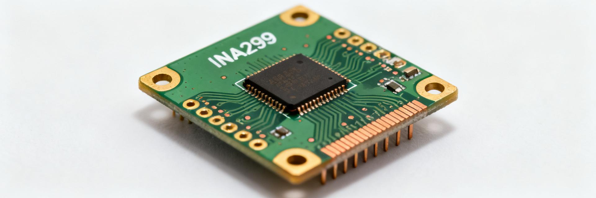
Key-purpose & operating envelope
The INA299 is a bidirectional small-signal amplifier optimized for high common-mode current sensing. Typical datasheet emphasis: supply range, maximum common-mode voltage, and allowable input differential. Engineers copy these values directly to confirm applicability before layout and purchase.
- Supply voltage range: 2.7 V to 5.5 V (example copy point).
- Maximum operating common-mode: up to ~80 V (operating limit row).
- Input differential range: limited to a few tens of millivolts without distortion.
Typical applications & selection criteria
Use this amplifier in high-side monitoring on power rails, battery systems, motor drives, and energy meters where bidirectional measurement and wide common-mode tolerance are required. Prefer it over discrete op-amp solutions when CM voltages exceed op-amp input range or when simplified gain options and integrated offsets reduce calibration effort.
| Specification Metric | Typical Operational Range | Worst-case Limit |
|---|---|---|
| Common-Mode Voltage (V_CM) | -4 V to 80 V | 85 V (Abs Max) |
| Supply Voltage (V_S) | 3.3 V to 5.0 V | 2.7 V to 5.5 V Range |
| Gain Configuration Options | 20 V/V, 50 V/V, 100 V/V | ±0.5% Maximum Error |
| Input Offset Voltage (V_OS) | ±35 µV | ±150 µV (Across Temp) |
Datasheet Deep-Dive #1 — Static electrical specs and accuracy
Input offset, gain error and accuracy budget
Point: build an accuracy budget from offset and gain error entries. Evidence: datasheet lists typical and worst-case offset voltage and gain error percentages. Explanation: convert offset volts to current error via the shunt: I_error_offset = V_offset / R_shunt, and convert gain error to % of full-scale current. Use worst-case sums for conservative design.
Common-mode range, CMRR, PSRR and survival limits
Point: operating CM range differs from survival rating—confirm both. Evidence: datasheet rows show CMRR in dB and survival tolerances in volts. Explanation: poor CMRR under large, noisy rails produces output error; PSRR indicates sensitivity to supply ripple. For high-side sensing, use operating CM headroom and survival margin to select transient protection and layout clearances.
Datasheet Deep-Dive #2 — Dynamic performance and electrical behavior
Bandwidth, slew rate, and stability
Point: bandwidth and slew limit transient fidelity. Evidence: datasheet lists small-signal bandwidth and slew rate per gain setting. Explanation: estimate step response time by t_r ≈ 0.35 / BW and check slew limits for large Vshunt steps. When selecting gain, remember higher gain often reduces bandwidth—trade measurement range against transient capture.
Noise, output drive, and thermal/power considerations
Point: noise sets low-current resolution; supply current drives thermal dissipation. Evidence: input-referred noise spectral density and supply current appear in electrical tables. Explanation: compute RMS noise by integrating noise density over system bandwidth; verify amplifier supply current times voltage stays within PCB thermal constraints and derating guidance in the datasheet.
Implementation Guide — How to design a reliable current-sense measurement with INA299
Choosing the shunt resistor and gain option (practical calculations)
Point: pick shunt and gain so Vout fits the ADC. Evidence: amplifier offers discrete gains (for example 20/50/100) and datasheet shows Vout swing. Explanation: target measurable current range → Vshunt = I × Rshunt → Vout = Gain × Vshunt. Example: for 0–50 A and a 5 mΩ shunt, Vshunt=0–0.25 V; with gain 20, Vout=0–5.0 V, fitting a 0–5 V ADC headroom while keeping margins for offset and clipping.
PCB layout, filtering and input protection best practices
Point: layout and input protection determine real-world accuracy. Evidence: datasheet recommends decoupling and input capacitance limits. Explanation: use Kelvin shunt traces, keep sense traces short, place decoupling caps close to the amplifier VCC pins, add an RC input filter (e.g., 100 Ω with 100 nF gives ~16 kHz corner) balancing noise and bandwidth, and include a bidirectional clamp for transient survival.
Practical Examples & Troubleshooting — Real measurements, test procedures and fixes
Example: measuring bidirectional current in a 48 V rail
Point: worked example for a 48 V high-side rail. Evidence: use a shunt and gain choice consistent with CM and ADC limits. Explanation: choose a 2 mΩ shunt for 0–20 A → Vshunt 0–40 mV; with gain 100, Vout 0–4.0 V; check ADC headroom and offset contribution: 100 μV offset → 50 mA error. Test procedure: verify with a scope, use differential probe or isolated measurement to capture step response and clipping.
Common pitfalls and datasheet-rooted fixes
Point: common failures map to specific specs. Evidence: clipping, CM-induced errors, thermal drift are frequent. Explanation: check output headroom rows if clipping occurs, confirm CMRR and PSRR if noise appears under load switching, and consult offset vs temperature tables when drift appears. Fixes include recalculating shunt, adding calibration coefficients, and improving layout or filtering.
Actionable Checklist & Design Pack — Pre-prototype checklist and next steps
Pre-prototype checklist
- Verify supply range and decoupling per datasheet recommendations.
- Confirm common-mode margin and survival voltage for worst-case transients.
- Calculate shunt power and temperature rise for continuous current loads.
- Choose gain to fit ADC input with headroom for offsets and calibration.
- Plan Kelvin routing, RC filter corners, and design appropriate test points.
What to validate in lab and what to document
Point: capture key measurements for design review. Evidence: datasheet plots to reproduce include offset vs temp, gain accuracy, noise spectra, and step response. Explanation: record offset across temperature, full-scale error, RMS noise in measurement bandwidth, and transient step response; document measured vs datasheet numbers and corrective calibration steps for traceability.
Summary
Key takeaways: watch accuracy budget entries, common-mode limits, available gain options, and bandwidth when interpreting the INA299 datasheet. Practical steps: compute shunt and gain so Vout fits the ADC, follow tight PCB layout rules, and run the checklist before prototype. Use the checklist above to validate your first prototype and record datasheet versus measured differences.
Key Summary
- Accuracy budget: convert offset and gain error to current error using I_error = V_offset / R_shunt and percent gain error against full scale.
- Common-mode: ensure operating CM and survival ratings exceed rail plus transient margin to avoid measurement distortion.
- Gain vs bandwidth: higher gain reduces bandwidth—pick gain to balance range and transient capture for your target signals.
FAQ — Common questions about INA299
How does the INA299 input offset affect current sense accuracy?
Input offset appears as a voltage added to the shunt voltage; divide that offset by the shunt resistance to get equivalent current error. For example, a 100 μV offset with a 2 mΩ shunt produces 50 mA error. Use datasheet worst-case offsets for conservative budgets and apply calibration to reduce residual error.
What common-mode limits should I check in the INA299 datasheet?
Confirm both the guaranteed operating common-mode range and the survival rating. The operating range ensures linear measurement; the survival rating indicates voltages the input can endure short-term. Design input clamps and spacing to keep the amplifier within operating limits under all expected transients.
How do I verify datasheet noise and bandwidth in the lab for INA299?
Measure input-referred noise by capturing output noise with a known gain and dividing by that gain, then integrate the spectral density across your system bandwidth to compute RMS noise. For bandwidth, apply a fast step to the shunt and measure output rise time; compare to t_r ≈ 0.35/BW calculated from the datasheet to confirm consistency.
How should the reference (REF) pin be configured for bidirectional sensing on the INA299?
Connect the REF pin to an external, stable voltage source (typically half of your dynamic ADC input range, such as V_REF/2). This level-shifts the zero-current voltage output, enabling the system to represent dynamic bidirectional current flows with accuracy.